
Mortgage or Cash: The Comparison That Matters

For wealthy families buying a home, the limit on the deductibility of mortgage interest is often well below the amount of financing they use. And now that we find ourselves in what may be a higher-for-longer rate environment, many are considering paying cash given the rate on a purchase mortgage looks high next to what those funds might earn invested. The decision is not as straightforward as it appears on the surface, from the standpoint of relative return, the deductibility of the interest, or the value of keeping that equity liquid. Here, I lay out what I believe to be a good framework for that decision-making process.
Two Problems, Same Tool
The first problem is the deduction. Interest on a home loan is deductible only on the first $750,000 of acquisition debt, and a home equity loan is not deductible at all. On a $2,000,000 house financed with a $1,500,000 mortgage, half the interest is simply lost. For the families this piece is written for, that is the normal case, not the exception.
The second problem is liquidity. Home equity is the least usable asset on most balance sheets. It earns nothing you can spend, it cannot be rebalanced, and getting it back out later means a new loan at whatever rate prevails then, with new costs, on the lender’s terms. A family that pays cash and later wants the money has given up the one moment when borrowing against the house was cheap and simple: at purchase.
The tool is the same in both cases. Borrow at purchase, or refinance after a cash closing once the rules below allow, invest the proceeds in a separate account built for the purpose, and treat the interest as investment interest rather than home mortgage interest. Done properly, the deduction is no longer capped, the equity is working, and the balance sheet keeps a liquid reserve outside the house.
The Comparison That Matters
Consider a hypothetical buyer with $1,000,000 in hand who can pay cash or borrow. If they pay cash, they invest what the payment would have been every month, and the comparison assumes they keep doing so for 30 years. If they take out a mortgage, they invest the $1,000,000 on day one and send the payments to the bank. Same dollars in, different timing.
A $1,000,000 loan is a jumbo mortgage in Orange County, Florida and in most of the country, since the 2026 conforming limit is $832,750. At today’s jumbo rate of 7.49%, the payment on $1,000,000 is $6,985 a month. If the portfolio also earns 7.49%, the lump sum grows to $9,393,487 over 30 years, and $6,985 a month invested at the same rate grows to $9,393,487. Equal to the dollar. The lump sum compounds harder, but the mortgage buyer pays $1,515,000 of interest along the way, and that interest is exactly the compounding advantage. So before tax, the loan rate is the breakeven.
Taxes break the tie. If three quarters of the interest is deductible at 37% and the refunds are invested, the mortgage buyer finishes about $1,850,000 ahead at that same 7.49% return. That is the government paying part of the interest, and it is why the structure in this piece exists.
But the breakeven is only the average. Returns do not arrive evenly, and the lump sum is exposed to every year of the next 30 while the monthly investor’s money mostly arrives late. The early years decide this bet.
What History Says
I ran both hypothetical scenarios through every month since April 1971, when Freddie Mac began publishing mortgage rates: a new window opens at every month-end, the loan is priced at the rate published that week, and both portfolios follow the S&P 500’s actual monthly total returns. Each point on the chart below represents the mortgage buyer’s advantage at the end of the window, as a percentage of the $1,000,000, before tax.
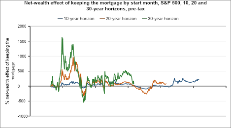
Net-wealth effect of keeping the mortgage by start month, S&P 500, 10, 20 and 30-year horizons, pre-tax
These results are back-tested and hypothetical; they do not represent any client account, and past performance is not indicative of future results.
| Horizon | Windows | Mortgage buyer wins | Median advantage | Worst case (start) | Median mortgage rate |
|---|---|---|---|---|---|
| 10 years | 546 | 73% | +49% | -96% (March 2000) | 7.79% |
| 20 years | 426 | 74% | +86% | -332% (May 1981) | 8.78% |
| 30 years | 306 | 86% | +275% | -548% (May 1981) | 9.58% |
The longer the horizon, the more often the mortgage buyer won, and the typical 30-year margin is large.
The failures come in two kinds. The buyer who borrowed in May 1981 paid about 17% and never caught up. The buyer who borrowed in March 2000 at 8.2% put the lump sum in at the top and, ten years later, held a portfolio worth less than the loan balance while the cash buyer feeding the payment into the same falling market finished about $960,000 ahead.
Over 30 years the portfolio’s annualized return beat the loan rate in only 56% of the windows, yet the mortgage buyer won 86% of the time, because strong early years compound on the lump sum for decades. Borrowing to invest is a bet on the first several years, and the 30-year average has much less to do with it. Said differently, timing and investment selection are important.
Few families would put the whole loan into the S&P 500, so here is the same test with a diversified portfolio alongside it, using an asset allocation mix of 25% S&P 500, 10% Russell 2000, 15% developed international, 5% emerging markets, 25% U.S. aggregate bonds, 5% Treasury bills, 5% high yield, 5% commodities, 5% REITs, and assumed to be rebalanced annually. The data for that mix begin in 2007, so the comparison covers ten-year windows starting June 2007 through September 2016.
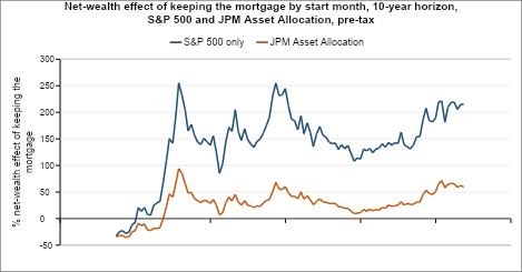
Net-wealth effect of keeping the mortgage by start month, 10-year horizon, S&P 500 and Asset Allocation, pre-tax
These results are back-tested and hypothetical; they do not represent any client account, and past performance is not indicative of future results.
The diversified buyer won 87% of those 112 windows by a median 30% of the loan, against 94% and 145% for the S&P 500 buyer, and both lost only when the loan was taken in the second half of 2007 with the crash a year away. Two cautions: loans in that period cost about 4%, far below today’s 7.49%, and a decade in which nothing beat U.S. stocks flatters the all-stock line. The diversified portfolio returned 6.3% a year over the period, below today’s loan rate; it won because the loan was cheap, not because it cleared 7.49%. At today’s rate, the portfolio has to be built to a higher standard than a conventional balanced mix, which is the subject of the next section.
The Tax Mechanism, and the Portfolio It Calls For
Interest on a loan secured by your home is normally home mortgage interest: deductible on the first $750,000 of acquisition debt, and not at all beyond that. If instead the proceeds go into a segregated investment account and stay there, the tax code lets you treat the interest as investment interest, deductible against investment income with no cap on the loan, and anything unused carries forward without expiration.
Three mechanics decide whether this works. A loan taken within 90 days of the purchase can be treated as acquisition debt, so either wait out the 90 days or make the election to treat the loan as not secured by the home, which is filed with the first year’s return and is effectively permanent. The proceeds must never mix with other money. And the deduction is only as good as the investment income available to absorb it: interest, ordinary dividends and short-term gains count in full, while qualified dividends and long-term gains count only if you give up their lower rate on the amount used.
That last point is what shapes the portfolio. Most taxable portfolios are built to avoid ordinary income because it could be subject to a marginal 37% federal income tax rate plus the 3.8% net investment income tax. With a deductible loan the arithmetic flips. Consider a hypothetical asset that earns 9% as ordinary income, financed at 7.49%. If the interest is not deductible you keep 9% less 40.8% tax, or 5.3%, against a 7.49% cost: a loss. Make the interest deductible at the same rate and you keep 59% of the 1.5 point spread: a gain. A nondeductible loan requires an ordinary-income asset to earn about 12.7% to break even; a deductible one requires 7.49%.
So the portfolio the structure calls for is different from the one most families already hold. It is weighted toward assets that produce taxable ordinary income and would not otherwise be worth owning in a taxable account, such as taxable bonds, private credit and hedge fund strategies taxed as ordinary income, alongside select equities. The loan interest shelters income that would otherwise be taxed at the highest rate, and those assets generate the investment income the deduction needs. Each part should be more likely than not to earn more than the loan costs after fees, and each part should move as little as possible with the others. That is what keeps a single bad stretch in one asset from deciding the outcome of the whole strategy. Finding those parts is a selection problem we work through with each family.
Liquidity, and a One-Sided Option
There is a reason to take the mortgage that has nothing to do with return. A 30-year fixed loan is the only long-term borrowing most families can get at a fixed rate with no covenants, no margin calls, and the right to pay it off whenever they choose. The equity stays liquid, in an account that can be rebalanced, drawn on, or used as collateral, rather than locked in the house until the next sale or the next loan application. Also, that liquidity does not need to be invested all at once.
The loan is also a one-sided option. If rates fall, you refinance and the breakeven drops for every year that remains. If rates rise, you keep 7.49% while new borrowers pay more and your fixed-rate liability loses value in real terms. Not every refinancing is the same: a lower rate on the same remaining term is a clean improvement; a lower rate with a new 30-year term is usually better still but is a fresh bet on the years it adds. Each one resets the Florida stamp and intangible taxes and has to be traced to the investment account the same way the original loan was.
Who This Fits
By my reading, four things decide it. Horizon: at ten years the two paths are close once taxes and costs are in; at 20 and 30 the mortgage buyer wins far more often than not. The portfolio: the proceeds must go into assets built to clear the loan rate after fees and stay invested through every downturn; if they would sit in cash or Treasuries, do not borrow. Cash flow: the buyer who borrowed in 2000 survived only because the mortgage payment came from employment income, not from selling assets into a falling market. And tax planning done before closing, not after; the 90-day rule, the election and the segregated account are not optional.
The case against, stated plainly: at today’s rate the pre-tax margin is thin, the outcome depends on years nobody can forecast, and the losses when it goes wrong are measured in multiples of the loan.
We work through this with each family individually. The numbers here are history, not a forecast.
Sources and Method
S&P 500 monthly total returns, April 1971 to September 2026, from FactSet: the S&P 500 total return index (SP50, gross, USD) from January 1988, which matches S&P Dow Jones Indices’ published calendar-year figures, and for 1971 to 1987 the FactSet S&P 500 price index with Robert Shiller’s monthly dividend data overlaid; the series matches Aswath Damodaran’s annual S&P 500 total returns to a mean difference of 0.24 points a year. Mortgage rates are the Freddie Mac Primary Mortgage Market Survey 30-year fixed rate, weekly, 1971-04-02 to 2026-10-08, from freddiemac.com/pmms, matched on every date to the FRED series MORTGAGE30US. The worked example uses the 30-year fixed jumbo contract rate from the Mortgage Bankers Association Weekly Applications Survey, 7.49% for the week ending October 9, 2026 (conforming was 7.50% in the same survey and 7.40% in Freddie Mac’s). The historical tests use the Freddie Mac conforming series because it is the only consistent weekly series back to 1971; jumbo loans priced above conforming for most of that history and at or slightly below it since about 2013, so the early-decade loan rates in the tests understate what a jumbo borrower would have paid. The diversified example uses FactSet Global Prices monthly total returns (USD, dividends reinvested) for exchange-traded fund proxies of the asset sleeves (SPY, IWM, EFA, EEM, AGG, BIL, HYG, DBC, VNQ), June 2007 to September 2026.
Method: a $1,000,000 30-year fully amortizing loan at the Freddie Mac rate nearest the start month-end, held fixed with no refinancing. The mortgage buyer invests $1,000,000 on day one and at the end of the window owes whatever balance remains. The cash buyer invests the monthly payment at the end of each month. Both portfolios compound at actual monthly returns; the diversified portfolio rebalances to target weights every 12 months. Results are nominal and before tax; neither buyer pays tax on portfolio returns in the model, which slightly favors the lump sum. With the portfolio return set equal to the loan rate, the two buyers finish identical in every window.
Tax rules referenced: Treasury Regulations 1.163-8T (interest tracing) and 1.163-10T(o)(5) (election), IRS Notice 88-74 (90-day rule), Internal Revenue Code section 163(d) (investment interest limit), IRS Publication 936, Florida Statutes 201.08 and 199.133. This piece is educational and is not tax or legal advice; the rules are applied to individual facts by your CPA.